Neural Networks From Linear Algebraic Perspective

Nowadays, I feel like machine learning is the most diverse academic field out there. I mean, you'll see people from so many different fields are getting involved and contributing here, statisticians, mathematicians, economists, neurologists, physicists, and so many others. Thanks to this diversity you'll see several interpretations of the same thing, people mumbling about probabilistic views, statistical views, mathematical views, etc. All of them have fascinated me, as it gives you perspective, lets you look at something in a different way.

The same goes for Neural Networks, which is arguably one of the most promising/dominating algorithms in machine learning at present and gave birth to its own field within ML, and that is Deep Learning. You can try understanding neural network's mysteries or the way it works in many ways, however, I've always enjoyed looking at it from the lenses of linear algebra, as it helps me to visualize the whole thing and build a mental picture. In this post, I aim to share some of those intuitions.

Neural Network 101:

In figure $1$, we can see a typical fully connected neural network, though the networks you will work with nowadays will be far deeper and complex than that, however, the intuition you'll build here can be applied to those as well. (Also, It's easier for me to explain using this simple case😁)

The basic training procedure of such a network for a classification task would be the following. A sample from the dataset gets feed into the network which is a column vector represented by $x$ in the figure, then we apply a linear transformation on $x$ which is simply a dot product between the vector $x$ and the weight matrix $W_h$ then we add a bias vector, thus, it now becomes an affine transformation of the input which ultimately gives us a vector that we pass through a non-linear function $f(.)$ and what we get is vector $a$ called the activations. To make it clearer, we can express the whole thing with the equation below:

After that, we repeat the same process, that is, passing $a$ through an affine transformation followed by another non-linear function sigmoid $\sigma(.)$ and we get our class prediction $\hat{y}$ (blue node at the end) from the network. It could be shown as the following:

We can write the whole thing that has been described above (Eqn. 1(a) and Eqn. 1(b)) with a single equation:

Voila! we're done with what we call the forward propagation of the network and in this post that's where we'll mostly concentrate on. So, let's just keep things simple for now.

Note: Till now, we've only performed a forward pass, there still remains a lot that goes into training a network, simply put, the network then uses a cost function to compute the loss, then with the help of backprop, It calculates the gradients and lastly, an optimizer such as SGD uses those gradients to update the parameters (weights) of the network. Maybe in a future post we can get deeper and talk about that stuff.

First, some intuitive talks:

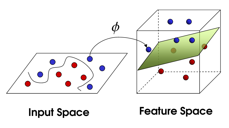
What is actually happening when we're applying a linear transformation to the input vector $x$ at eqn. 1(a)? If you remember from your linear algebra classes when you multiply a vector by a matrix, the resultant vector is a linear combination of the columns of the matrix, which can also be thought of as a weighted sum of the columns of the matrix. Let's say our weight matrix is of shape $3$x$2$ (where $3$ is the number of nodes in the hidden layer and $2$ is the number of nodes in the input layer), consequently, the shape of input vector $x$ is $2$x$1$ ($2$ dimensional input), thus the shape of the vector we would get after the dot product would be $3$x$1$ ($3$ dimensional output). Did you see that, the weight matrix has "placed" our input from a 2D to a 3D space. So, with a matrix of such shape (num. hidden layer nodes > num. input layer nodes) we can change the representation space of our input by projecting it onto a higher dimension, In this case, a higher dimension is not a curse but a blessing as it gives the optimizer more freedom to move around. Now, the other advantage that we get after the matrix-vector multiplication is that it can transform the input data in several ways. Depending on the matrix, it can rotate, reflect, shear, and scale the data. If we look closely there's one type of transformation missing which is the translation (rigid vertical/horizontal movement of data points). To make it happen we include the bias term at eqn. 1(a), so now, from linear transformation ($W_hx$) it becomes what we call an affine transformation ($W_hx + b$). Let's make the whole thing a bit clearer with some visuals.

I've made a moon-shaped dataset with $2$ classes (red and purple) which is not linearly separable (figure 2), that is you can't do a good job at separating $2$ classes with a straight line. Here, the data points lie in $\R^2$ space and each point has $2$ features, its x-coordinate value, and y-coordinate value. so our input vector shape would be $2$x$1$ (It's $x$,$y$ value). Now let's see what happens to the dataset after we perform both linear transformation and affine transformation using a matrix of shape $2$x$2$ (means we shall remain in 2D after transformation, so that we can plot the data points and investigate the changes).

figure 3(a): Linear Transformation

figure 3(b): Affine Transformation

As can be seen from figure 3(a), with the linear transformation ($W_hx$) data points got transformed while remaining at the origin so no translation, but in figure 3(b), It's clear that with the affine transformation ($W_hx + b$), along with scaling and a bit of other transformations data points got translated as well.

let's make things more explicit:

In figure 4, we can see the whole thing about the operation of the network in a nice illustrated way. here each connection (represent by colored lines) that goes from input to hidden layer (pink to green) is an element/value of the weight matrix. For simplification purposes we've excluded the bias term and non-linearity, also we're only considering the first $2$ layers that's why the rest of the network has been muted. Now, let's come back to the discussion, till now we were talking from a macroscopic view when we were saying "performing dot product between weight matrix and input vector" but let's dig a bit deeper and peek into dot products from a microscopic view. I think we've all learned the dot product rule at the very beginning of our linear algebra course, so what we do is we take a row vector from the matrix and then simply multiply it with the column vector at hand that gives us a scalar and it is the first element of the resultant vector, we perform this operation for each row of the matrix. So, what we're doing is actually performing a bunch of scalar products between $2$ vectors, right? (a row vector from the weight matrix and the input column vector). So, let's move onto vector dot-products now.

We've taken the first row vector named $w_1$ from the weight matrix $W_h$ (figure 4) and performed dot product with the input column vector $x$. As we can see from figure 5 the formula that we use for dot product has a term that includes the cosine angle between the vectors, which means if the $2$ vectors are orthogonal then the dot product value would be $0$ ($cos 90° = 0$), similarly, other cases have been mentioned in figure 5 as well. So, it's evident that the dot product value would be the highest when the $2$ vectors are closest in space (means they are parallel and the cosine angle is zero, as we know $cos 0° = 1$) and it would be the lowest when they're pole apart (means both are in the opposite direction and cosine angle between them is $180°$, as we know $cos 180° = -1$). Thus, the result of the dot product is also called similarity score in ML lingo. In the deep learning community, people love dot product because it's too simple yet tells so much as we just saw.

So, we've come to the understanding that the dot product of $2$ vector tells us their degree of alignment or how similar they are, that means when we're multiplying weight matrix $W_h$ with input vector $x$ (figure 4), we're checking the degree of alignment between $x$ and each row vector of $W_h$, this is also known as template matching/kernel matching which is another powerful idea and lingo you may have heard when working with CNNs. In CNN, we take each kernel which can be thought of as a "long-flat" column vector and perform dot product with a patch of the input image (which can also be thought of as a "long-flat" column vector). When the network is trained, each kernel learns a particular feature of the input, say for example a kernel has learned the "nose" feature of the human face, so whenever there is a nose in the picture and that kernel performs dot product over the input image's nose patch, then it produces a really high value (as we've just seen, their similarity score would be high), that's how it detects the nose.

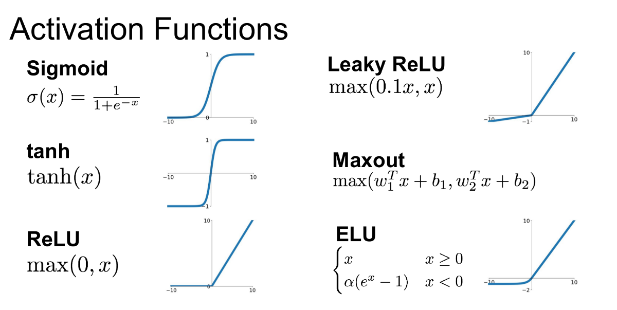
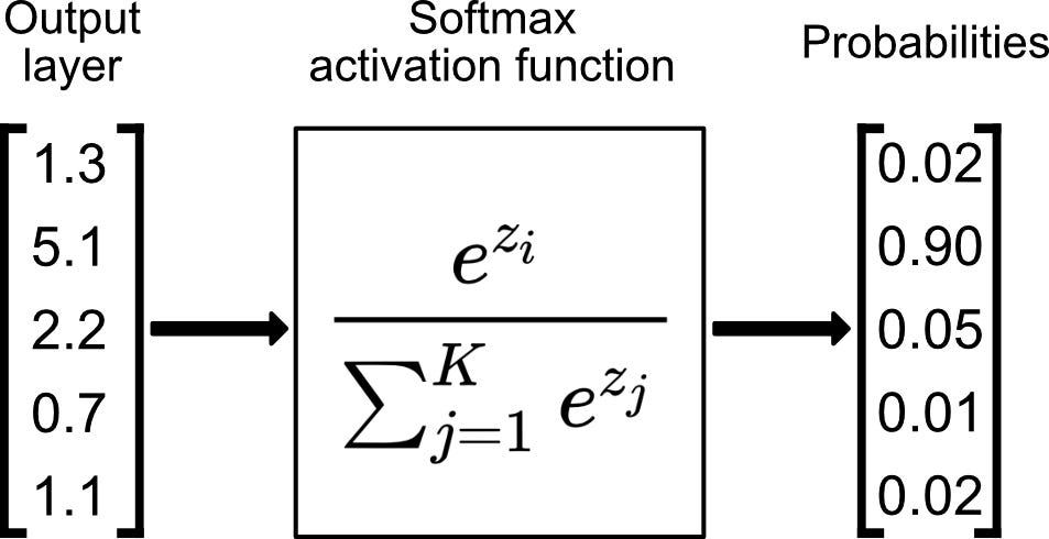
Note: We haven't really talked about non-linearity, which is a really important and necessary part because it is what lets the network create complex mappings between the input and output. Our linear transformation alone can't make it happen, as we remain in the linear space even after many many linear transformations are applied (e.g. $W_4(W_3(W_2(W_1x))) = Wx$). In practice, we mostly use the function $(.)^+$called ReLU as non-linearity, which is a piecewise linear function. There're other functions as well you may use depending on your task such as hyperbolic tangent, sigmoid, softmax, etc. As we've described above, linear transformation rotates/scales/shears... our data, likewise We can think of non-linearities as it squashes the data, it'll help to create the mental picture that we were talking about.

Now, let's peek inside:

We've done a lot of theory, now it's time to see those things applied in action. Remember that we saw a moon shape non-linearly separable dataset in figure 2? In this section we'll train a neural net and see if it can pull the $2$ somewhat entangled classes apart with all the transformational stuff that it can do like "Rotation, Scaling, Shearing, Reflecting, Translation" (affine transformation) and "Squashing" (non-linear transformation).

To do this, I've made the following network -

1. Input Layer (2D)
2. Hidden Layer (100D) --> $Tanh()$
3. Embedding Layer (2D) --> $Tanh()$
4. Output Layer (1D) --> $sigmoid()$

Here, the embedding layer is used to plot the data, as our hidden layer is 100D (which we can't obviously plot) thus it has been projected onto a lower dimension (2D) so that we can plot it down, it's a neat trick to let your neural network do the PCA for you😉. Also, I've used Tanh() as non-linearity in hidden layers.

Now let's start training the model, we'll train it for $150$ epochs, and we're hoping at the beginning the network may perform poorly but as it gets trained It will able to separate $2$ classes by applying transformations, placing it to a higher dimension and squashing.

figure 6(a): Network is applying various transformations to make data linearly separable

figure 6(b): Network is learning decision boundary

Both in figure 6(a) and in 6(b) we can see two perspectives of the training phase of the network. In figure 6(b) the network is learning the complex decision boundary. But figure 6(a) is my favorite as here we can witness the things we've covered above is actually being applied. The network at the beginning makes arbitrary transformations (which is obvious, as in the beginning our weight matrix is initialized with random values), thus the classifier placed in the last layer is unable to separate the $2$ classes with a hyperplane (straight line in $2$D), but then as the weight matrix gets updated (also thanks to the non-linearity) the transformations become more and more meaningful and at the very end of the animation we can see points of distinct classes gets totally separated, that's when the classifier is actually able to separate the $2$ classes with a hyperplane which then becomes the curvy decision boundary of figure 6(b).

look at this image to see how a hyperplane becomes a curve.

Conclusion:

The concepts of linear algebra are very rich and intuitive, with the help of those concepts we can break down such a complex system like neural networks and understand its inner workings. It's difficult for us to think beyond 3-4 dimensions, however, with help of linear algebra, we can travel through $100$s of dimensions and even higher because all it takes is just a matrix multiplication.

Acknowledgments:

Thank you to Rosanne Liu, Alfredo Canziani and my faculties Chowdhury Rafeed Rahman, Swakkhar Shatabda for their feedbacks and word of encouragements.

• Alfredo Canziani's intuitions on these topics helped me a lot to see things in this manner and also his open-sourced codes helped me to create the plots.
• Just like many others, Chris Olah has inspired me as well with his incredibly intuitive posts and it's one of the reasons I made this blog.
• Last but not the least, my faculty Sajid Ahmed who has always motivated me and literally spoonfed the basics of ML.

Please hit me up on twitter or comment below for any feedback or corrections.